Week 17 Tips for using dplyr
Here are a few handy resources with more detail on wrangling with dplyr and tidyr:
As is the case in many software packages, there is always more than one way to get something done in R! Base-R tools can accomplish all kinds of tasks, but sometimes they are cumbersome and inefficient.
Because most of our use of R as epidemiologists is focused on the tools of data science, you might find the diverse and continually evolving tidyverse a great toolbox to explore. Originated by Hadley Wickham (founder of RStudio), the packages constituting the tidyverse are now contributed by lots of different people. What they have in common is an interest in handling data in tidy ways. R for Data Science is an authoritative guide to tidy data, and many of the tools constituting the tidyverse including ggplot2, dplyr and more.
This appendix is a very brief introduction to the dplyr package which is a set of data manipulation functions. In other words it is the epidemiologists’ go-to package for data manipulation, recoding, and preparation in R.
There are two high-level observations about how we will use dplyr this semester:
-
dplyrfunctions can be thought of as verbs. That means each one is a tool to act on your data, producing a change. So your question is “what do I want to change?” - Functions in
dplyr(and in many other parts of thetidyversefor that matter) can be stand alone code. Or alternatively they can be chained together in a sequence. This chaining (called piping because the tool to connect or chain steps is called a pipe and looks like this:%>%) can make your code both easier for humans to read, and also helps run a sequence of steps more efficiently.
For the examples below, I will use the Georgia motor vehicle crash mortality dataset where the unit of observation (e.g. the content of one row of data) is a Georgia county, and the columns are variable names. This dataset is also explicitly spatial meaning that it includes geography information regarding the boundaries of each county, contained with the geom column, as is typical for sf class data in R.
Here is what the first few rows of the dataset looks like (minus the geom column):
## Reading layer `ga_mvc' from data source
##   `/Users/mkram02/Library/CloudStorage/OneDrive-EmoryUniversity/EPI563-Spatial Epi/SpatialEpi-2021/DATA/GA_MVC/ga_mvc.gpkg'
##   using driver `GPKG'
## Simple feature collection with 159 features and 17 fields
## Geometry type: MULTIPOLYGON
## Dimension:     XY
## Bounding box:  xmin: -85.60516 ymin: 30.35785 xmax: -80.83973 ymax: 35.00066
## Geodetic CRS:  WGS 84
## GEOID NAME variable estimate County
## 1 13001 Appling County, Georgia B00001_001 1504 Appling County
## 2 13003 Atkinson County, Georgia B00001_001 875 Atkinson County
## 3 13005 Bacon County, Georgia B00001_001 945 Bacon County
## 4 13007 Baker County, Georgia B00001_001 390 Baker County
## 5 13009 Baldwin County, Georgia B00001_001 2943 Baldwin County
## 6 13011 Banks County, Georgia B00001_001 1767 Banks County
## MVCDEATHS_05 MVCDEATHS_14 MVCDEATH_17 TPOP_05 TPOP_14 TPOP_17
## 1 4 4 10 17769 18540 18521
## 2 5 1 3 8096 8223 8342
## 3 7 5 0 10552 11281 11319
## 4 1 1 1 3967 3255 3200
## 5 6 8 13 46304 45909 44906
## 6 4 8 6 16683 18295 18634
## NCHS_RURAL_CODE_2013 nchs_code rural MVCRATE_05 MVCRATE_14 MVCRATE_17
## 1 6 Non-core Rural 22.51111 21.57497 53.99276
## 2 6 Non-core Rural 61.75889 12.16101 35.96260
## 3 6 Non-core Rural 66.33813 44.32231 0.00000
## 4 4 Small metro non-Rural 25.20797 30.72197 31.25000
## 5 5 Micropolitan non-Rural 12.95784 17.42578 28.94936
## 6 6 Non-core Rural 23.97650 43.72779 32.19921
17.1 select()
The first verb of dplyr is called select() and it is useful when you want to remove or select specific columns/variables. For instance, as mentioned this dataset has 17 attribute columns plus the geom column. But perhaps we only need three variables, and we decided it would be easier to exclude the unneeded variables? Then we can select() those we want (or inversely we can select those we don’t want).
There are three useful tips on using select() with spatial data:
- To select variables to keep simply list them (e.g.
select(data, var1, var2, var3)) - If it is easier to only omit specific variables (e.g. perhaps you have 100 variables and you only want to drop 3), place a negative sign before the name (e.g.
select(data, -var5, -var6)). - Finally, something specific to working with
sfspatial data is that the geometry column (typically namedgeomorgeometry) is sticky. That means that it’s hard to get rid of it. That’s actually a good thing. You usually want the geometry to stick with the attribute data. But occasionally you might want to convert you spatialsfdata object into an aspatialdata.frame. To do this you must first set the geometry to be null like this:aspatial.df <- st_set_geometry(spatial.df, NULL). See additional info here.
Let’s do that with the motor vehicle crash data.
# First we read in the dataset, which is stored as a geopackage
mvc <- st_read('GA_MVC/ga_mvc.gpkg')

# Look at column names
names(mvc)

# For this example we do not want the geom column because it is too big to view
mvc2 <- st_set_geometry(mvc, NULL)

# Creating a new object with only 4 attributes
mvc2 <- select(mvc2, GEOID, NAME, rural, MVCRATE_05, MVCRATE_17)

# look at column names
names(mvc2)
## [1] "GEOID" "NAME" "variable"
## [4] "estimate" "County" "MVCDEATHS_05"
## [7] "MVCDEATHS_14" "MVCDEATH_17" "TPOP_05"
## [10] "TPOP_14" "TPOP_17" "NCHS_RURAL_CODE_2013"
## [13] "nchs_code" "rural" "MVCRATE_05"
## [16] "MVCRATE_14" "MVCRATE_17" "geom"## [1] "GEOID" "NAME" "rural" "MVCRATE_05" "MVCRATE_17"
17.2 mutate()
Another frequently needed verb is called mutate() and as you might guess it changes your data. Specifically mutate() is a function for creating a new variable, possibly as a recode of an older variable. The mvc data object has 159 rows (one each for n=159 counties).
Let’s imagine that we wanted to create a map that illustrated the magnitude of the change in the rate of death from motor vehicle crashes between 2005 and 2017. To do this we want to create two new variables that we will name delta_mr_abs (the absolute difference in rates) and delta_mr_rel (the relative diference in rates).
# Now we make a new object called mvc2
mvc3 <- mutate(mvc2,
               delta_mr_abs = MVCRATE_05 - MVCRATE_17,
               delta_mr_rel = MVCRATE_05 / MVCRATE_17)
If you look at the help documentation for mutate() you’ll see that the first argument is the input dataset, in this case mvc. Then anywhere from one to a zillion different ‘recode’ steps can be included inside the parentheses, each separated by a comma. Above, we created two new variables, one representing the absolute and the other representing the relative difference in rates between the two years.
We can look at the first few rows of selected columns to see the new variables:
head(mvc3)## GEOID NAME rural MVCRATE_05 MVCRATE_17 delta_mr_abs
## 1 13001 Appling County, Georgia Rural 22.51111 53.99276 -31.481650
## 2 13003 Atkinson County, Georgia Rural 61.75889 35.96260 25.796294
## 3 13005 Bacon County, Georgia Rural 66.33813 0.00000 66.338135
## 4 13007 Baker County, Georgia non-Rural 25.20797 31.25000 -6.042034
## 5 13009 Baldwin County, Georgia non-Rural 12.95784 28.94936 -15.991517
## 6 13011 Banks County, Georgia Rural 23.97650 32.19921 -8.222703
## delta_mr_rel
## 1 0.4169284
## 2 1.7173090
## 3 Inf
## 4 0.8066549
## 5 0.4476038
## 6 0.7446303
17.3 filter()
While select() above was about choosing which columns you keep or drop, filter() is about choosing which rows you keep or drop. If you are more familiar with SAS, filter() does what an if or where statement might do.
Imagine we wanted to only map the urban counties, and omit the rural counties. We could do this be defining a filtering rule. A rule is any logical statement (e.g. a relationship that can be tested in the data and return TRUE or FALSE).
Here we create a new dataset, mvc4 that is created from mvc3 but is restricted only to non-Rural counties:
mvc4 <- filter(mvc3, rural == 'non-Rural')


dim(mvc3) # dimensions (rows, columns) of the mvc3 object
## [1] 159 7
dim(mvc4) # dimensions (rows, columns) of the restricted mvc4 object## [1] 102 7As you can see the original object (mvc3) had 159 rows, while the filtered object (mvc4) has only 102, reflecting the number of non-Rural counties in Georgia.
Although the example above used only one filtering rule (e.g. keep only rows where rural == 'non-Rural'), you could construct a complex filter by including several different logical tests within the filter() function, each separated by a comma. For instance you could filter for non-rural counties with a population above 100,000 and in a specified region of the state, assuming you had variables indicating each of those values.
17.4 arrange()
Occasionally you might want to sort a dataset, perhaps to find the lowest or highest values of a variable, or to group like values together. Sorting with dplyr uses the arrange() verb. By default, data is arranged in ascending order (either numerical or alphabetical for character variables), but you can also choose descending order as below:
##   GEOID                     NAME     rural MVCRATE_05 MVCRATE_17 delta_mr_abs
## 1 13307  Webster County, Georgia     Rural   38.81988  115.16315    -76.34327
## 2 13269   Taylor County, Georgia     Rural   22.57336   73.69197    -51.11860
## 3 13165  Jenkins County, Georgia     Rural   47.00353   57.03205    -10.02853
## 4 13001  Appling County, Georgia     Rural   22.51111   53.99276    -31.48165
## 5 13087  Decatur County, Georgia non-Rural   18.17455   52.40305    -34.22851
## 6 13191 McIntosh County, Georgia non-Rural   16.11863   49.62427    -33.50564
##   delta_mr_rel
## 1    0.3370859
## 2    0.3063205
## 3    0.8241598
## 4    0.4169284
## 5    0.3468223
## 6    0.3248135
17.5 %>% Pipe operator
Everything we’ve done up until now has been one step at a time, and we created five different datasets to avoid overwriting our original. But one source of coding efficiency in R comes from the careful chaining or piping together of multiple steps.
While every verb above required an input dataset as the first argument, when we chain steps, the functions take the output of the previous step as the input for the current step. For example this code chunk does everything we did above in one step:
mvc6 <- mvc %>%
  st_set_geometry(NULL) %>%                             # remove geom column
  select(GEOID, NAME, rural, MVCRATE_05, MVCRATE_17) %>%# select target variables
  mutate(delta_mr_abs = MVCRATE_05 - MVCRATE_17,        # recode variables
        delta_mr_rel = MVCRATE_05 / MVCRATE_17) %>%
  filter(rural == 'non-Rural') %>%                      # filter (restrict) rows
  arrange(desc(MVCRATE_17))                             # sort by MVCRATE_17

dim(mvc6)
## [1] 102 7
head(mvc6)## GEOID NAME rural MVCRATE_05 MVCRATE_17 delta_mr_abs
## 1 13087 Decatur County, Georgia non-Rural 18.17455 52.40305 -34.228506
## 2 13191 McIntosh County, Georgia non-Rural 16.11863 49.62427 -33.505640
## 3 13033 Burke County, Georgia non-Rural 34.87510 39.96093 -5.085824
## 4 13189 McDuffie County, Georgia non-Rural 18.67501 37.21276 -18.537756
## 5 13055 Chattooga County, Georgia non-Rural 11.76194 36.33428 -24.572337
## 6 13227 Pickens County, Georgia non-Rural 29.32874 34.82335 -5.494612
## delta_mr_rel
## 1 0.3468223
## 2 0.3248135
## 3 0.8727301
## 4 0.5018442
## 5 0.3237147
## 6 0.8422147In practice, it takes some experience to write a whole chain of steps that do what you want. I often go iteratively, adding one step at a time and checking that each step is doing what I expected.
17.6 group_by() and summarise()
A dplyr verb that can be incredibly important for spatial epidemiology is the combination of group_by() with summarise(). These two are used to aggregate and summarize data. For instance if you had data arranged with individual persons as the unit of analysis (e.g. 1 person = 1 row of data), but you wanted to aggregate them so you got counts per census tract, you could use group_by() to arrange the rows into groups defined by census tract, and then use summarise() to do some calculation (e.g. count, mean, sum, etc) separately for each group.
In fact, you can enter multiple variables into the group_by() argument and the result is the cross-classification of grouping. For example, imagine you had COVID-19 line listing data where each row is a single person, and rows include age (young or old) as well as county of residence. If you enter group_by(county, age) the data will be stratified by age within county. If you then used summarise(count = n()), you would get a count of individual cases in each age group and in each county. You could use this to make a map of the density of young and old cases by county.
An important feature of sf data objects when operated on by dplyr verbs, is that there is built in functionality to handle geography/geometry data. So for instance, imagine we wanted to create a map where we aggregated all of the rural counties and separately all of the non-rural counties.
mvc7 <- mvc %>%
  group_by(rural) %>%
  summarise(avg_mr_17 = mean(MVCRATE_17))

mvc7 %>% st_set_geometry(NULL)
## # A tibble: 2 × 2
## rural avg_mr_17
## * <chr> <dbl>
## 1 Rural 29.2
## 2 non-Rural 18.8As you can see (and as you might have predicted), the aggregation changed our dataset from 159 rows to 2 rows: one row for rural and one for non-rural. Let’s see what it did to the spatial data by first mapping the original data, and then mapping the aggregated data. Read more about qtm()) and other tmap functions.
# Using the qtm() function from tmap to create map of original data
m1 <- qtm(mvc, 'MVCRATE_17')

# Using the qtm() function from tmap package to create a map
m2 <- qtm(mvc7, 'avg_mr_17')

tmap_arrange(m1, m2)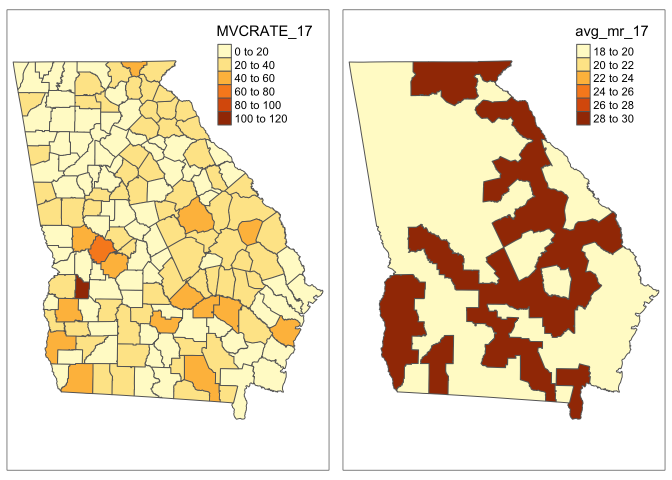
As with other dplyr verbs (e.g. mutate(), select(), filter()), you are not constrained to using group_by() with only a single variable. Returning to the example with individual observations nested within census tracts, you could use new_data <- individ_data %>% group_by(gender, year, tract) to create a file that has a row of data for each unique stratum of gender * year * census tract.
You may see a message in the R console when you run group_by() followed by summarise() that says something like summarise() ungrouping output override with .groups argument. What this is telling you is that R automatically ungrouped your data. More specifically it removed grouping by the last group_by() variable, to avoid unintended consequences from persistent grouping. If you group_by() two or more variables it only drops the last grouping*, so other grouping may persist. All grouping can be removed by adding ungroup() after the summarise().
17.7 join()
Merging data is so common in epidemiology, but also prone to so many unintended consequences that it is important to pay attention to the options for successful merges or ‘table joins’ as they are called in the parlance of relational databases.
Because of the challenges with getting the desired output from a merge or join(), dplyr has a set of verbs including: left_join(), right_join(), inner_join(), full_join() and more. Here is documentation of the many ways to join!
A join is simply a way to merge two tables when they have some common key or ID variable. For our purposes in this class I want to focus on several key features of joining that are important for spatial analysis.
For this explanation we will work with two separate files: an aspatial data.frame with the motor vehicle crash data called mvc.df; and a sf object of all U.S. counties, called us. The unit of analysis in each is the county, there is a common ID or key variable in the county FIPS code (named GEOID), but they have a different number of rows:
dim(mvc.df) # this is dimensions for the aspatial attribute data## [1] 159 17
dim(us) # this is dimensions for the spatial county polygon sf data## [1] 3221 13As expected, the mvc.df has the \(n=159\) counties that makeup Georgia. However the spatial/geography information has \(n=3220\) rows, corresponding to the number of U.S. counties and territories.
First, the difference between the xxxx_join() is how the two tables relate to one another. For most purposes a left_join() or right_join() will do the trick. Here is the difference: a left_join() starts with the first object and joins it to the second. In contrast the right_join() starts with the second object and joins it to the first. What does that mean?
# left join, starting with mvc.df as the first object, us as the second
test.left <- mvc.df %>%
  left_join(us, by = 'GEOID')

dim(test.left)
## [1] 159 29
class(test.left)## [1] "data.frame"
# right join, starting with mvc.df as the first object
test.right <- us %>%
  left_join(mvc.df, by = 'GEOID')

dim(test.right)
## [1] 3221 29
class(test.right)## [1] "sf" "data.frame"What did we learn?
- The number of rows in the output dataset is dictated by two things:
- the order the objects are written (e.g. in this case
mvc.dfwas always first anduswas always second, contained within thejoin()) - the direction of the join. In a
left_join()the merge begins withmvc.df, which limits the output to only 159 rows. In contrast withright_join()the merge begins withus, which limits the output to 3220 rows. - The class of the output data depends on which object was first. Notice that in the
left_join(), because we started with an aspatialdata.frame, the output is also an aspatialdata.frame(although thegeomcolumn is now incorporated!). In contrast with theright_join()which put thesfobjectusfirst, the class wassf.
This means that when merging or joining you should think about whether you want all of the rows of data to go to the output, or only some; and think about whether (or how) you can make the sf object be first.
In the scenario above, we only want \(n=159\) rows, and thus want to exclude all of the non-Georgia counties. That means we must have mvc.df first. Therefore, we could force the object to be of class sf like this (also see info here):
## [1] 159 29
class(test.left)## [1] "sf" "data.frame"Joining when Key/ID variables have different names
Sometimes we have a common variable, such as the county FIPS code, but the variable names are different. For example in the code below, the column storing the unique county ID for the mvc.df is named GEOID. However the column in the sf object us that stores the unique county ID is named FIPS. It is still possible to use the join() verbs by relating them (inside a c() concatenation) in the order in which the datasets are introduced.
17.8 Reshaping (transposing) data
There are numerous other intermediate to advanced data manipulation options available in dplyr and the tidyverse, but most are outside of the scope of this course. One final verb that represents a more sophisticated kind of data change, is however useful in preparing spatial data. That is the tools to transpose or reshape a rectangular dataset from wide to long or vice versa. Transposing is useful when, for example, you have a column with a disease rate for each of several years (these data are wide), but you want a dataset where a single column contains the rate and a separate column indicates the year (these data are long). This article introduces the notion of pivoting data; you can also review this section in R for Data Science
Two related verbs help pivot tidy data one direction or the other:
17.8.1 pivot_longer() for going from wide to long
Reviewing the article linked in the previous paragraph (or searching the help documentation) will give you more detail. But as an example we will look at how to take our current mvc dataset, which contains the motor vehicle crash mortality rate for each county from three different years (2005, 2014, 2017) as separate columns (e.g. it is wide):
# this code shows the first 6 rows (the head) of the relevant variables
mvc %>%
  st_set_geometry(NULL) %>%
  select(GEOID, NAME, MVCRATE_05, MVCRATE_14, MVCRATE_17) %>%
  head()
## GEOID NAME MVCRATE_05 MVCRATE_14 MVCRATE_17
## 1 13001 Appling County, Georgia 22.51111 21.57497 53.99276
## 2 13003 Atkinson County, Georgia 61.75889 12.16101 35.96260
## 3 13005 Bacon County, Georgia 66.33813 44.32231 0.00000
## 4 13007 Baker County, Georgia 25.20797 30.72197 31.25000
## 5 13009 Baldwin County, Georgia 12.95784 17.42578 28.94936
## 6 13011 Banks County, Georgia 23.97650 43.72779 32.19921For mapping a time-series it is often beneficial to have the data long, which is to say we want the data with a single column for mvc_rate and a separate column for year, and then we can choose to create a map for each subset (defined by year) of the data.
mvc_long <- mvc %>%
  select(GEOID, NAME, MVCRATE_05, MVCRATE_14, MVCRATE_17) %>%
  as_tibble() %>%
  pivot_longer(cols = starts_with("MVCRATE"),
               names_to = c(".value", "year"),
               values_to = "mvc_rate",
               names_sep = "_") %>%
  mutate(year = 2000 + as.numeric(year)) %>%
  st_as_sf()
First let’s look at the results, and then I’ll walk through each of the steps in the code chunk above:
mvc_long %>%
  st_set_geometry(NULL) %>%
  head()
## # A tibble: 6 × 4
## GEOID NAME year MVCRATE
## <chr> <chr> <dbl> <dbl>
## 1 13001 Appling County, Georgia 2005 22.5
## 2 13001 Appling County, Georgia 2014 21.6
## 3 13001 Appling County, Georgia 2017 54.0
## 4 13003 Atkinson County, Georgia 2005 61.8
## 5 13003 Atkinson County, Georgia 2014 12.2
## 6 13003 Atkinson County, Georgia 2017 36.0As you can see, we now have 3 rows for Appling County (GEOID 13001): one for each of the three years, with different MVCRATE in each. That is a long dataset. So how did that code work? Here is a step-by-step of what that code chunk did:
- The first step was to create a new object,
mvc_longthat will be the outcome of all of the steps piped together. The input to the pipe is the original dataset,mvc. - The use of
as_tibble()is a current work around to an annoying ‘feature’ of thepivot_*functions and that is that they don’t play well withsfdata classes. So when we useas_tibble()we are essentially removing the class designation, (making it atibblewhich is a tidy object); importantly this is different fromst_set_geometry(NULL)which actually omits the geometry column (e.g. see additional detail here). - I used
select()to pull out only the variables of interest, although you could leave other variables if desired. -
pivot_longer()can be called in several ways. The way I call it here, I first specified which columns to pivot by defining thecols =argument to be all variables that start with the phraseMVCRATE.starts_with()is another utility function indplyr. So this step toldRthat the columns I wanted changed were the three calledMVCRATE_05,MVCRATE_12andMVCRATE_17 - The
names_to =argument defines the column name in the new dataset that will delineate between the three variables (e.g.MVCRATE_05, etc). In our case we wanted the value to be the year not the wordMVCRATE_12. To accomplish this we had to do some extra work:
- First, note that we used the option
names_sep = '_'. That is another utility function that says we want to break a string into parts wherever a designated separated (e.g. the underscore,_) occurs. So this will take the column nameMVCRATE_05and break it at the underscore to return two parts:MVCRATEand05. - Because breaking it into two would produce two answers, we had to make two variable names in the
names_to =to hold them. Thusnames_to = c(".value", "year"). In other words the column labeled.variablewill hold the valueMVCRATEand the columnyearwill hold the value05 -
'.value'is actually a special value in this instance. It is a way of designating that the first part was essentially junk. As such it will automatically be discarded.
-
values_to = 'mvcrate'. This is where we define the name in the new dataset that will hold the actual value (e.g. the MVC mortality rate itself.) - The
mutate()step is just a way to take the year fragment (e.g.05,12,17) and make it into calendar years by first making it numeric, and then simply adding 2000. - The final step,
st_as_sf()is because all of the manipulations above actually removed the objects designation as classsf. Importantly, it DID NOT remove thegeomcolumn, but the object is not recognized (e.g. bytmap) as a spatial object. Sost_as_sf()simply declares that it is in factsf.
The best way to wrap your head around this is to start trying to reshape or transpose data you have on hand. You may need to look for additional help or examples online, but with time it will become more intuitive.
To see why you might have gone through all of that work, we will use the tm_facets() (read more abouttmap_facets() here).
tm_shape(mvc_long) +

  tm_fill('MVCRATE') +
  tm_borders() +
tm_facets(by = 'year')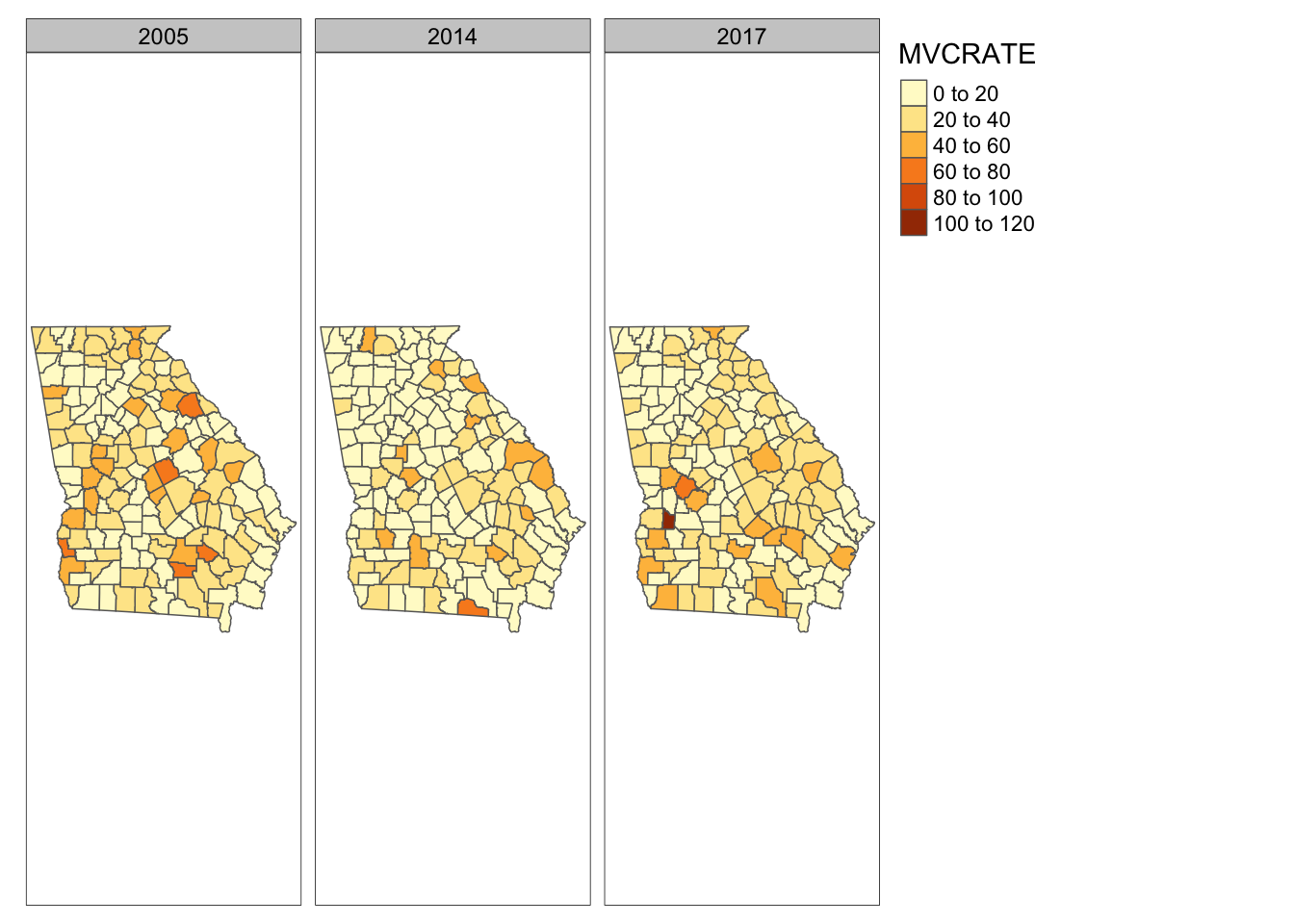
17.8.2 pivot_wider()
Of course it is also possible to go the other way, from long to wide. This often is easier. Here is some code to return to our original shape:
mvc_wide <- mvc_long %>%
  as_tibble() %>%
  mutate(my_var = paste0('MVCRATE ', year)) %>%
  select(-year) %>%
  pivot_wider(names_from = my_var,
              values_from = MVCRATE) %>%
  st_as_sf()
Take a look at the output:
mvc_wide %>%
  st_set_geometry(NULL) %>%
  head()
## # A tibble: 6 × 5
## GEOID NAME `MVCRATE 2005` `MVCRATE 2014` `MVCRATE 2017`
## <chr> <chr> <dbl> <dbl> <dbl>
## 1 13001 Appling County, Georgia 22.5 21.6 54.0
## 2 13003 Atkinson County, Georgia 61.8 12.2 36.0
## 3 13005 Bacon County, Georgia 66.3 44.3 0
## 4 13007 Baker County, Georgia 25.2 30.7 31.2
## 5 13009 Baldwin County, Georgia 13.0 17.4 28.9
## 6 13011 Banks County, Georgia 24.0 43.7 32.2It appears that we have returned to 1 row per county. So what were all of those steps?
- Once again, we start by removing the class designation
sfbut callingas_tibble() -
mutate()is called to re-create a variable that will become the column names. - We no longer need the old
yearvariable so I omit it withselect(-year) - Finally the
pivot_wider()call has arguments defining which current variable contains the informatino that will be the new column name (names_from =) and which current variable contains the information that will population the cells within that column (values_from =).