Week 1 Locating Spatial Epidemiology

1.1 Getting Ready

1.1.1 Learning objectives

TABLE 1.1: Learning objectives by weekly module

After this module you should be able to…
Explain the potential role of spatial analysis for epidemiologic thinking and practice.
Produce simple thematic maps of epidemiologic data in R.

1.1.2 Additional Resources

• Geocomputation with R by Robin Lovelace. This will be a recurring ‘additional resource’ as it provides lots of useful insight and strategy for working with spatial data in R. I encourage you to browse it quickly now, but return often when you have questions about how to handle geographic data (especially of class sf) in R.
• An introduction to the ggplot2 package. This is just one of dozens of great online resources introducing the grammar of graphics approach to plotting in R.
• A basic introduction to the tmap package This is also only one of many introductions to the tmap mapping package. tmap builds on the grammar of graphics philosophy of ggplot2, but brings a lot of tools useful for thematic mapping!
• R for SAS users cheat sheet

1.1.3 Important Vocabulary

TABLE 1.2: Vocabulary for Week 1

Term	Definition
Data, attribute	Nonspatial information about a geographic feature in a GIS, usually stored in a table and linked to the feature by a unique identifier. For example, attributes of a county might include the population size, density, and birth rate for the resident population
Data, geometry	Spatial information about a geogrpahic feature. This could include the x, y coordinates for points or for vertices of lines or polygons, or the cell coordinates for raster data
Datum	The reference specifications of a measurement system, usually a system of coordinate positions on a surface (a horizontal datum) or heights above or below a surface (a vertical datum)
Geographic coordinate system	A reference system that uses latitude and longitude to define the locations of points on the surface of a sphere or spheroid. A geographic coordinate system definition includes a datum, prime meridian, and angular unit
Geopackage	A data storage format suitable for containing vector or raster data in a compact and portable file. It is an alternative (and in my opinion a superior alternative!) to ESRI shapefiles.
Projection	A method by which the curved surface of the earth is portrayed on a flat surface. This generally requires a systematic mathematical transformation of the earth's graticule of lines of longitude and latitude onto a plane. Some projections can be visualized as a transparent globe with a light bulb at its center (though not all projections emanate from the globe's center) casting lines of latitude and longitude onto a sheet of paper. Generally, the paper is either flat and placed tangent to the globe (a planar or azimuthal projection) or formed into a cone or cylinder and placed over the globe (cylindrical and conical projections). Every map projection distorts distance, area, shape, direction, or some combination thereof
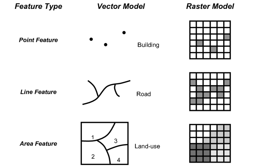
Spatial data model: raster	A spatial data model that defines space as an array of equally sized cells arranged in rows and columns, and composed of single or multiple bands. Each cell contains an attribute value and location coordinates. Unlike a vector structure, which stores coordinates explicitly, raster coordinates are contained in the ordering of the matrix. Groups of cells that share the same value represent the same type of geographic feature (see Figure below)
Spatial data model: vector	A coordinate-based data model that represents geographic features as points, lines, and polygons. Each point feature is represented as a single coordinate pair, while line and polygon features are represented as ordered lists of vertices. Attributes are associated with each vector feature, as opposed to a raster data model, which associates attributes with grid cells (see figure below)
Unit of analysis	The unit or object that is measured, analyzed, and about which you wish to make inference. Examples of units of analysis are person, neighborhood, city, state, or hospital.

1.2 Spatial Thinking in Epidemiology

When first learning epidemiology, it can be difficult to distinguish between the concepts, theories, and purpose of epidemiology versus the skills, tools, and methods that we use to implement epidemiology. But these distinctions are foundational to our collective professional identity, and to the way we go about doing our work.

For instance, do you think of epidemiologists as data analysts, scientists, data scientists, technicians or something else? These questions are bigger than we can address in this class, but their importance becomes especially apparent when learning an area such as spatial epidemiology. This is because there is a tendency for discourse in spatial epidemiology to focus primarily on the data and the methods without understanding how each of those relate to the scientific questions and health of population for which we are ultimately responsible. Distinguishing these threads is an overarching goal of this course, even as we learn the data science and spatial analytic tools.

One quite simplistic but important example of how our questions and methods are inter-related is apparent when we think of data. Data is central to quantitative analysis, including epidemiologic analysis. So how is data different in spatial epidemiology?

1.2.1 Unit of analysis

The first thing that might come to mind is that in this course and your related future spatial epi work, there is explicitly geographic or spatial measures contained within our data. The content of the spatial data is distinct: the addition of geographic or spatial location may illuminate otherwise aspatial attributes. But even more fundamental than the content is thinking about the unit of analysis.

It is likely that in many other examples in your epidemiology coursework, the explicit (or sometimes implicit) unit of analysis has been the individual person. Spatial epidemiology can definitely align with individual-level analysis. But as we will see, common units we observe and measure in spatial epidemiology – and therefore the units that compose much of our data – are not individuals but instead are geographic units (e.g. census tract, county, state, etc) and by extension the collection or aggregation of all the individuals therein.

This distinction in unit of analysis has important implications for other epidemiologic concerns including precision, bias, and ultimately for inference (e.g. the meaning we can make from our analysis), as we’ll discuss throughout the semester.

One concrete implication of the above discussion is that you should always be able to answer a basic question about any dataset you wish to analyze: “what does one row of data represent?” A row of data is one way to think of the unit of analysis, and often (but not always) in spatial epidemiology a row of data is a summary of the population contained by a geographic unit or boundary.

Said another way it is an ecologic summary of the population. As stated above, this is only the most simplistic example of how and why it is important to not only learn the spatial statistics and methods, but to also maintain the perspective of epidemiology as a population health science. To advance public health we need good methods but we also need critical understanding of the populations we support, the data we analyze, and the conclusions we can reliably draw from our work.

As we move through the semester, I encourage you to dig deep into how methods work, but also to step back and ask questions like “Why would I choose this method?” or “What question in epidemiology is this useful for?”

1.3 Spatial Analysis in Epidemiology

1.3.1 Spatial data storage formats

If you have worked with spatial or GIS data using ESRI’s ArcMap, you will be familiar with what are called shapefiles. This is one very common format for storing geographic data on computers. ESRI shapefiles are not actually a single file, but are anywhere from four to eight different files all with the same file name but different extensions (e.g. .shp, .prj, .shx, etc). Each different file (corresponding to an extension) contains a different portion of the data ranging from the geometry data, the attribute data, the projection data, an index connecting it all together, etc.

What you may not know is that shapefiles are not the only (and in my opinion definitely not the best) way to store geographic data. In this class I recommend storing data in a format called geopackages indicated by the .gpkg extension.

Geopackages are an open source format that were developed to be functional and portable across devices, including mobile devices. They are useful when we are storing individual files in an efficient and compact way.

To be clear, there are many other formats and I make no claim that geopackages are the ultimate format; they just happen to meet the needs for this course, and for much of the work of spatial epidemiologists. It is worth noting that many GIS programs including ArcMap and QGIS can both read and write the geopackage format; so there is no constraint or limitation in terms of software when data are stored in .gpkg format.

1.3.2 Representing spatial data in R

The work in this course assumes that you are a basic R user; you do not need to be expert, but I assume that you understand data objects (e.g. data.frame, list, vector), and basic operations including sub-setting by index (e.g. using square brackets to extract or modify information: []), base-R plotting, and simple regression modeling. If you are not familiar with R, you will need to do some quick self-directed learning.

Here are some good online resources for R skills, and the instructor and TA’s can point you to additional resources as needed:

• The Epidemiologist R Handbook
• R for Data Science, particularly the introductory chapters
• R Tutorial

Just as our conceptualization of, or thinking about, data in spatial epidemiology requires some reflection, the actual structure and representation of that data with a computer tool such as R also requires some attention.

Specifically, spatial data in R is not automatically the same as conventional aspatial epidemiologic data that is often arranged as a rectangular data.frame (e.g. like a spreadsheet where rows are observations and columns are variables).

While spatial data are more complex than just a spreadsheet, it does not need to be as complex as spatial data in software platforms like ESRI’s ArcMap.

To be spatial, a dataset must have a representation of geography, spatial location, or spatial relatedness, and that is most commonly done with either a vector or raster data model (see description above in vocabulary). Those spatial or geographic representations must be stored on your computer and/or held in computer memory, hopefully with a means for relating or associating the individual locations with their corresponding attributes. For example, we want to know the attribute (e.g. the count of deaths for a given place), and the location of that place, and ideally we want the two connected together.

Over the past 10+ years, R has increasingly been used to analyze and visualize spatial data. Early on, investigators tackling the complexities of spatial data analysis in R developed a number of ad hoc, one-off approaches to these data. This worked in the short term for specific applications, but it created new problems as users needed to generalize a method to a new situation, or chain together steps. In those settings it was not uncommon to convert a dataset to multiple different formats to accomplish a task sequence; this resulted in convoluted and error-prone coding, and lack of transparency in analysis.

An eventual response to this early tumult was a thoughtful and systematic approach to defining a class of data that tackled the unique challenges of spatial data in R. Roger Bivand, Edzer Pebesma and others developed the sp package which defined spatial data classes, and provided functional tools to interact with them.

The sp package defined specific data classes to contain or represent points, lines, and polygons, as well as raster/grid data. Each of these data classes can contain geometry only (these have names like SpatialPoints or SpatialPolygons) or could contain geometry plus related data attributes (these have names like SpatialPointsDataFrame or SpatialPolygonsDataFrame).

Each spatial object can contain all the information spatial data might include: the spatial extent (min/max x, y values), the coordinate system or spatial projection, the geometry information, the attribute information, etc.

Because of the flexibility and power of the sp* class of objects, they became a standard up until the last few years. Interestingly, it was perhaps the sophistication of the sp* class that began to undermine it. sp* class data was well-designed from a programming point of view, but was still a little cumbersome (and frankly confusing) for more applied analysts and new users.

Analysis in spatial epidemiology is not primarily about computer programming, but about producing transparent and reliable data pipelines to conduct valid, reliable, and reproducible analysis. Thus, epidemiologists and other data scientists desired spatial tools that could be incorporated into the growing toolbox of data science tools in R.

These calls for a more user-friendly and intuitive approach to spatial data led the same team (e.g. Bivand, Pebesma, others) to develop the Simple Features set of spatial data classes for R. Loaded with the sf – for simple features – package, this data format has quickly become the standard for handling spatial data in R.

The power of the sf class, as discussed below, is that it makes spatial data behave like rectangular data and thus makes it amenable to manipulation using any tool that works on data.frame or tibble objects. Recognizing that many users and functions prefer the older sp* objects, the sf package includes a number of utility functions for easily converting back and forth.

In this class we will use sf* class objects as the preferred data class, but because some of the tools we’ll learn have not been updated recently and thus still require sp*, we will occasionally go back and forth.

sf* data classes are designed to hold all the essential spatial information (projection, extent, geometry), but do so with an easy to evaluate data.frame format that integrates the attribute information and the geometry information together. The result is more intuitive sorting, selecting, aggregating, and visualizing.

1.3.3 Benefits of sf data classes

As Robin Lovelace writes in his online eBook, Gecomputation in R, sf data classes offer an approach to spatial data that is compatible with QGIS and PostGIS, important non-ESRI open source GIS platforms, and sf functionality compared to sp provides:

1. Fast reading and writing of data
2. Enhanced plotting performance
3. sf objects can be treated as data frames in most operations
4. sf functions can be combined using %>% pipe operator and works well with the tidyverse collection of R packages (see Tips for using dplyr for examples)
5. sf function names are relatively consistent and intuitive (all begin with st_)

1.3.4 Working with spatial data in R

Here and in lab, one example dataset we will use, called ga.mvc quantifies the counts and rates of death from motor vehicle crashes in each of Georgia’s \(n=159\) counties. The dataset is vector in that it represents counties as polygons with associated attributes (e.g. the mortality information, county names, etc).

1.3.4.1 Importing spatial data into R

It is important to distinguish between two kinds of data formats. There is a way that data is stored on a computer hard drive, and then there is a way that data is organized and managed inside a program like R.

The shapefiles (.shp) popularized by ESRI/ArcMap is an example of a format for storing spatial data on a hard drive. In contrast, the discussion above about the sf* and sp* data classes refer to how data is organized inside R.

Luckily, regardless of how data is stored on your computer, it is possible to import almost any format into R, and once inside R it is possible to make it into either the sp* or sf* data class. That means if you receive data as a .shp shapefile, as a .gpkg geopackage, or as a .tif raster file, each can be easily imported.

All sf functions that act on spatial objects begin with the prefix st_. Therefore to import (read) data we will use st_read(). This function determines how to import the data based on the extension of the file name you specify.

Look at the help documentation for st_read(). Notice that the first argument dsn=, might be a complete file name (e.g. myData.shp), or it might be a folder name (e.g. mygeodatabase.gdb). So if you had a the motor vehicle crash data saved as both a shapefile (mvc.shp, which is actually six different files on your computer), and as a geopackage (mvc.gpkg) you can read them in like this:

# this reads in the shapefile
mvc.a <- st_read('GA_MVC/ga_mvc.shp')

# this reads in the geopackage
mvc.b <- st_read('GA_MVC/ga_mvc.gpkg')

We can take a look at the defined data class of the imported objects within R:

class(mvc.a)

## [1] "sf"         "data.frame"

class(mvc.b)

## [1] "sf"         "data.frame"

Notice how the two objects have the same class (e.g. type of data stored within R), even though they were two different kinds of files stored on the computer: one was a shapefile and one a geopackage. This is because st_read() can automatically detect the storage format based on the extension, and use the appropriate interpreter to import that data. This is nice because it means you can bring many types of spatial data into R!

You will also notice that when we examined the class() of each object, they are each classified as both sf and data.frame class. That is incredibly important, and it speaks to an elegant simplicity of the sf* data classes!

That the objects are classified as sf is perhaps obvious because it is a spatial object; but the fact that each object is also classified as data.frame means that we can treat the object for the purposes of data management, manipulation and analysis as a relatively simple-seeming object: a rectangular data.frame.

How does that work? We will explore this more in lab but essentially each dataset has rows (observations) and columns (variables). We can see the variable/column names like this:

names(mvc.a)

## [1] "GEOID"      "NAME"       "MVCRATE_17" "geometry"

names(mvc.b)

## [1] "GEOID"      "NAME"       "MVCRATE_17" "geom"

We can see that each dataset has the same attribute variables (e.g. GEOID, NAME, MVCRATE_17), and then a final column called geometry in one and called geom in another.

These geometry columns are different from your usual run-of-the-mill column variables in that they don’t hold a single value. Instead, each ‘cell’ in those columns actually contains an embedded list of \(x,y\) coordinates defining the vertices of the polygons for each of Georgia’s counties. So all of the spatial location information for each row is contained in that single variable called geom (or alternately, geometry).

Another way to learn about an sf object is to use the head() function. In addition to displaying the top six rows of data (which is the typical behavior of the head() function), for sf objects head() will also print some of the important metadata about the file.

head(mvc.a)

## Simple feature collection with 6 features and 3 fields
## Geometry type: MULTIPOLYGON
## Dimension:     XY
## Bounding box:  xmin: -84.64195 ymin: 31.0784 xmax: -82.04858 ymax: 34.49172
## Geodetic CRS:  WGS 84
##   GEOID                     NAME MVCRATE_17                       geometry
## 1 13001  Appling County, Georgia   53.99276 MULTIPOLYGON (((-82.55069 3...
## 2 13003 Atkinson County, Georgia   35.96260 MULTIPOLYGON (((-83.141 31....
## 3 13005    Bacon County, Georgia    0.00000 MULTIPOLYGON (((-82.62819 3...
## 4 13007    Baker County, Georgia   31.25000 MULTIPOLYGON (((-84.64166 3...
## 5 13009  Baldwin County, Georgia   28.94936 MULTIPOLYGON (((-83.42674 3...
## 6 13011    Banks County, Georgia   32.19921 MULTIPOLYGON (((-83.66862 3...

To summarize, sf within R is powerful because:

1. We are not limited to how data arrive to us. If you acquire data (from the web, a colleague, etc) as a shapefile, a geopackage, a raster or other formats, they can all be imported into R.
2. Once inside of R (and stored in sf data objects), we can treat the datasets almost as if they were aspatial, rectangular datasets. That means we could use sub-setting, filtering, recoding, merging, and aggregating without losing the spatial information!

1.3.4.2 Exporting spatial data from R

While importing is often the primary challenge with spatial data and R, it is not uncommon that you might modify or alter a spatial dataset and wish to save it for future use, or to write it out to disk to share with a colleague.

Luckily the sf package has the same functionality to write an sf spatial object to disk in a wide variety of formats including shapefiles (.shp) and geopackages (.gpkg). Again, R uses the extension you specify in the filename to determine the target format.

# Write the file mvc to disk as a shapefile format
st_write(mvc, 'GA_MVC/ga_mvc_v2.shp')

# Write the file mvc to disk as a geopackage format
st_write(mvc, 'GA_MVC/ga_mvc_v2.gpkg')

After you write the two files, navigate on your computer to the folder and look at what was written. In particular notice that the .shp file is actually many files, but the .gpkg is a single file.

1.3.5 Basic visual inspection/plots

What if you want to see your spatial data? In base-R there is a powerful function called plot() that can be used to create easy or incredibly complex visualizations or graphical representation of data.

In the package sf, the functionality of plot() is extended to handle the uniqueness of spatial data. That means that if you call plot() on a spatial object without having loaded sf, the results will be different than if plot() called after loading sf.

When you plot() with sf, by default it will try to make a map for every variable in the data frame! Try it once. If this is not what you want (it usually is not), you can force it to only plot some variables by providing a vector of variable names.

plot(mvc) # this plots a panel for every column - or actually the first 10 columns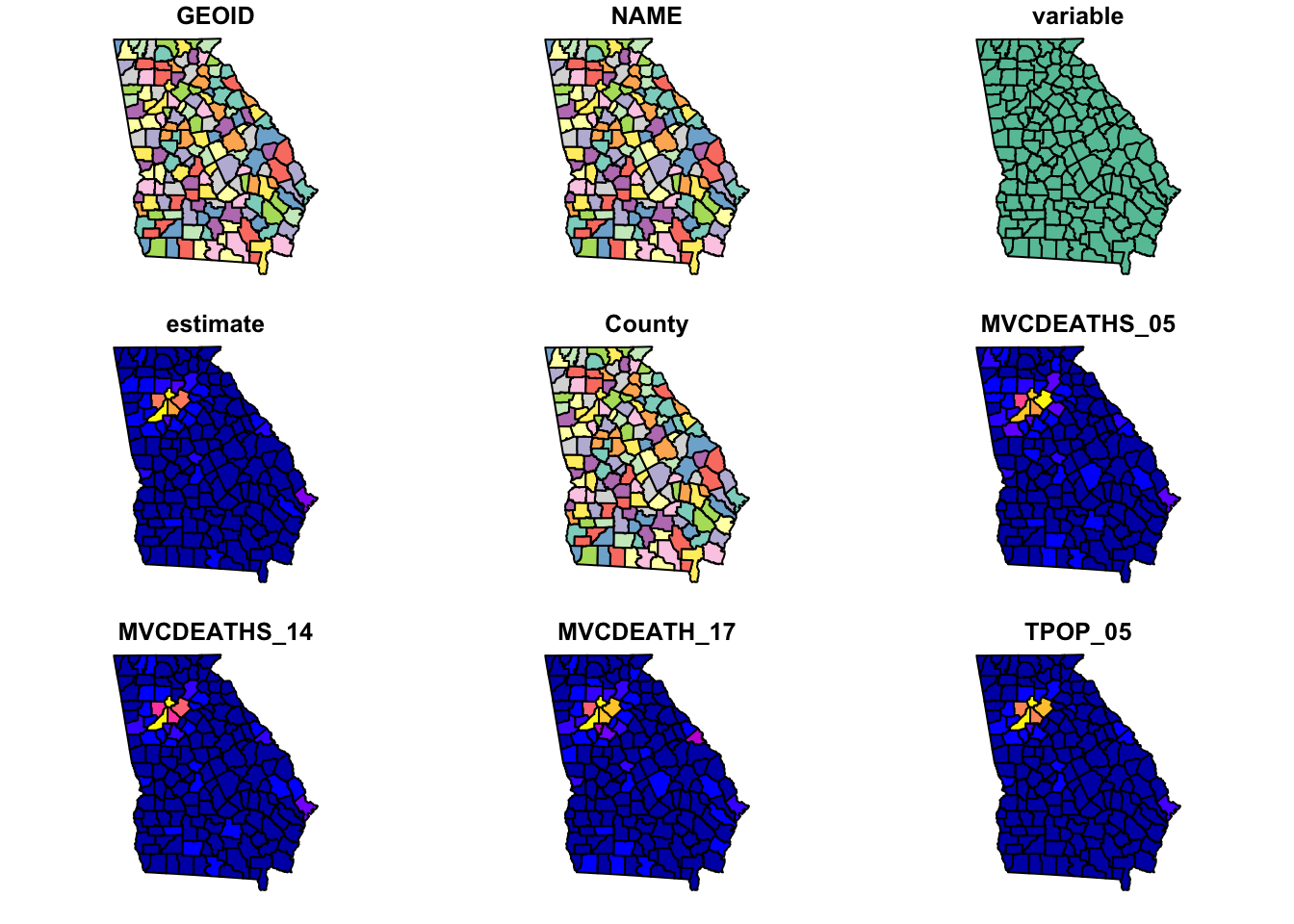

plot(mvc['MVCRATE_05']) # this plots only a single variable, the MVC mortality rate for 2005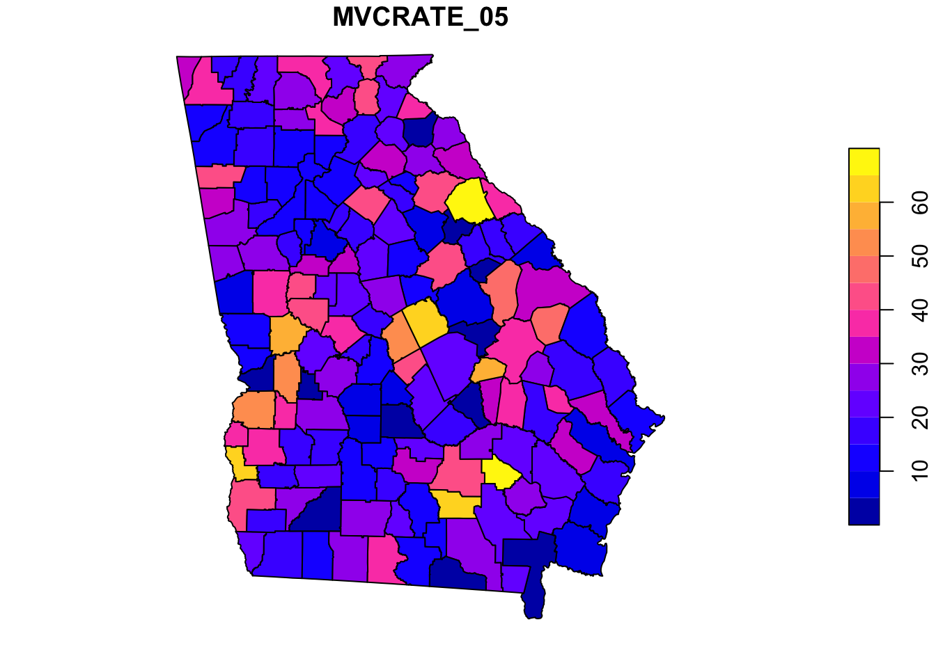

plot(mvc[c('MVCRATE_05', 'MVCRATE_17')]) # this plots two variables: MVC rate in 2005 & 2017

Sometimes you want to know something about the spatial size, extent, or shape of your data. To do this you can easily plot only the geometry of the spatial object (e.g. not attributes). Here are two approaches to quickly plot the geometry:

plot(st_geometry(mvc)) # st_geometry() returns the geom information to plot

plot(mvc$geom)  # this is an alternative approach...directly plot the 'geom' column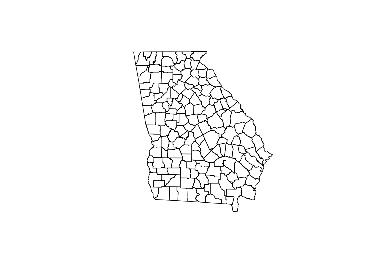

1.3.6 Working with CRS and projection

Maps are used to describe the geographical or spatial location of particular objects as a representation of where those things are on planet Earth. Most maps are printed on paper or screens. In other words, maps identify locations from somewhere on planet earth and represent them on a flat or planar medium.

But the world does not have latitude or longitude lines painted on the ground, and the earth is not flat! Instead the earth is nearly spherical (really it is a geoid) and there is no universal reference for where to start measuring.

For these two reasons, all maps require at a minimum a coordinate reference system (CRS) to define how the numbers in our coordinates relate to actual places. In addition most maps are best interpreted after formally projecting the data to account for the artifact induced by pretending earth is flat.

The most unambiguous way to describe a CRS and/or projection is by using the EPSG code, which stands for European Petroleum Survey Group. This consortium has standardized hundreds of projection definitions in a manner adopted by several R packages including rgdal and sf.

A given dataset already has a CRS (and possibly a projection). If CRS and projection information was contained in the original file you imported, it will usually be maintained when you use st_read(). However sometimes it is missing and you must first find it. Once it is known, you might choose to change or transform the CRS or projection for a specific purpose. We will discuss this further in class.

If there is NO CRS information imported it is critical that you find out the CRS information from the data source or owner.

This course is not a GIS course (e.g. it is assumed you have already had some exposure to geographic information systems generally), and learning about the theory and application of coordinate reference systems and projections is not our primary purpose this semester. However, some basic knowledge is necessary for successfully working with spatial epidemiologic data. Here are several resources you should peruse to learn more about CRS, projections, and EPSG codes:

• A useful overview/review of coordinate reference systems in R
• Robin Lovelace’s Geocompuation in R on projections with sf
• EPSG website: This link is to a searchable database of valid ESPG codes
• Here are some useful EPSG codes

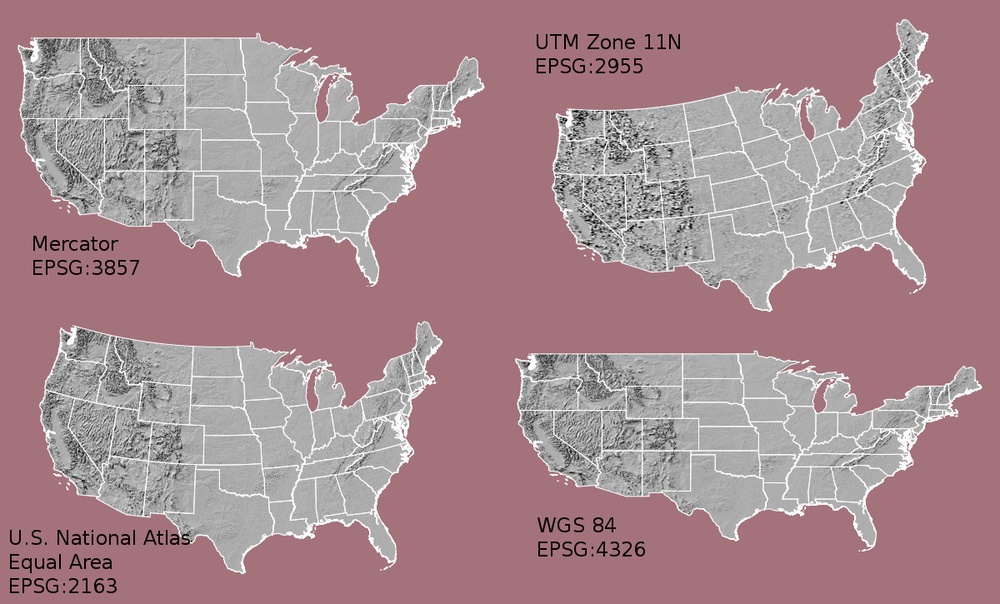
FIGURE 1.1: Comparing CRS

The choice of CRS and/or projection has a substantial impact on how the rendered map looks, as is evident in the figure above (source of image).

We already saw the CRS/projection information of the mvc object when we used the head() function above; it was at the top and read WGS 84.

Recall there are two main types of CRS:

1. Geographic which is to say coordinate locations are represented as latitude and longitude degrees;
2. Projected which means the coordinate values have been transformed for representation of the spherical geoid onto a planar (Euclidean) coordinate system.

WGS 84 is a ubiquitous geographic coordinate system common to boundary files retrieved from the U.S. Census bureau.

An important question when you work with a spatial dataset is to understand whether it is primarily a geographic or projected CRS, and if so which one.

st_is_longlat(mvc)

## [1] TRUE

This quick logical test returns TRUE or FALSE to answer the question “Is the sf object simply a longitude/latitude geographic CRS?”. The answer in this case is TRUE because WGS 84 is a geographic (longlat) coordinate system, and there is no additional information about projection. But what if it were FALSE or we wanted to know more about the CRS/projection?

# Retrieve CRS metadata from an sf object
st_crs(mvc)

## Coordinate Reference System:
##   User input: WGS 84 
##   wkt:
## GEOGCRS["WGS 84",
##     ENSEMBLE["World Geodetic System 1984 ensemble",
##         MEMBER["World Geodetic System 1984 (Transit)"],
##         MEMBER["World Geodetic System 1984 (G730)"],
##         MEMBER["World Geodetic System 1984 (G873)"],
##         MEMBER["World Geodetic System 1984 (G1150)"],
##         MEMBER["World Geodetic System 1984 (G1674)"],
##         MEMBER["World Geodetic System 1984 (G1762)"],
##         MEMBER["World Geodetic System 1984 (G2139)"],
##         ELLIPSOID["WGS 84",6378137,298.257223563,
##             LENGTHUNIT["metre",1]],
##         ENSEMBLEACCURACY[2.0]],
##     PRIMEM["Greenwich",0,
##         ANGLEUNIT["degree",0.0174532925199433]],
##     CS[ellipsoidal,2],
##         AXIS["geodetic latitude (Lat)",north,
##             ORDER[1],
##             ANGLEUNIT["degree",0.0174532925199433]],
##         AXIS["geodetic longitude (Lon)",east,
##             ORDER[2],
##             ANGLEUNIT["degree",0.0174532925199433]],
##     USAGE[
##         SCOPE["Horizontal component of 3D system."],
##         AREA["World."],
##         BBOX[-90,-180,90,180]],
##     ID["EPSG",4326]]

This somewhat complicated looking output is a summary of the CRS stored with the spatial object. There are two things to note about this output:

• At the top, the User input is WGS 84
• At the bottom of the section labeled GEOGCRS it says ID["EPSG",4326"]

While there are literally hundreds of distinct EPSG codes describing different geographic and projected coordinate systems, for this semester there are three worth remembering:

• EPSG: 4326 is a common geographic (unprojected or long-lat) CRS
• EPSG: 3857 is also called WGS 84/Web Mercator, and is the dominant projection used by Google Maps
• EPSG: 5070 is the code for a projected CRS called Albers Equal Area which has the benefit of representing the visual area of maps in an equal manner.

One rule of thumb to determine if data are in degrees of lat/long (and thus geographic) versus in linear units such as meters or miles (and thus projected) is to look at the xmin, ymin, xmax, and ymax that are printed at the top of the output whenever you use head(xxx).

Degrees of latitude (the y-axis values) will range from \(-90^\circ\) to \(+90^\circ\), and degrees of longitude (the x-axis values) will range from \(0^\circ\) to \(180^\circ\).

In contrast most projected data will have cartesian or linear units (rather than degrees), usually with numbers much higher than 180.

Once the CRS/projection is clearly defined, you may choose to transform or project the data to a different system. The sf package has another handy function called st_transform() that takes in a spatial object (dataaset) with one CRS and outputs that object transformed to a new CRS.

# This uses the Albers equal area USA, 
mvc.aea <- st_transform(mvc, 5070)

# This uses the Web Mercator CRS (EPSG 3857) which is just barely different from EPSG 4326
mvc.wm <- st_transform(mvc, 3857)

# Now let's look at them side-by-side
plot(st_geometry(mvc), main = 'EPSG 4326')
plot(st_geometry(mvc.wm), main = 'Web Mercator (3857)')
plot(st_geometry(mvc.aea), main = 'Albers Equal Area (5070)')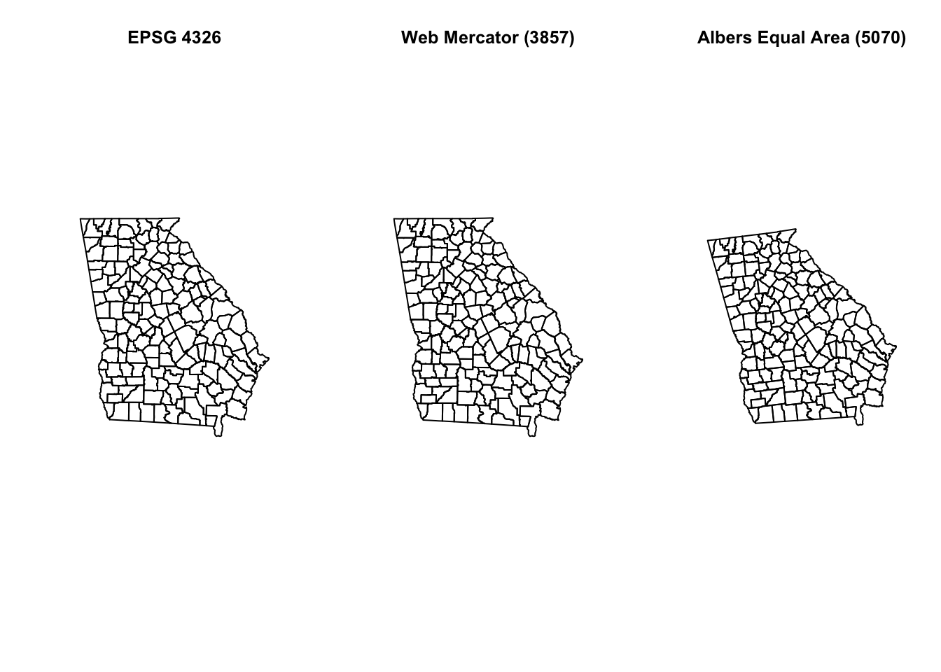

Do you see some difference between the three? Although EPSG 4326 is unprojected and EPSG 3857 is projected (e.g. Mercator is a conical projection), they appear similar, although not identical.

Mercator projection is known to have increased distortion further from the equator. In general we will prefer to use ‘projected’ rather than ‘unprojected’ (long/lat only) data for both visualization and analysis, and more specifically we almost always prefer equal area projections for choropleth maps, because the coloring of the area being represented communicates something about intensity of the measure.

Whenever you bring in a new dataset you will need to check the CRS and project or transform it as needed.

Important: It is important to distinguish between defining the current projection of data and the act of projecting or transforming data from one known system to a new CRS/projection.

We cannot transform data until we correctly define its current or original CRS/projection status. The above function tells us what the current status is. In some cases data do not have associated CRS information and this might be completely blank (for instance if you read in numerical \(x,y\) points from a geocoding or GPS process).

In those cases you can set the underlying CRS using st_set_crs() to attach a user-known definition to the data object, but this assumes you know what it is.

There are two arguments to this function: the first is x = objectName, and the second is value = xxx where ‘xxx’ is a valid EPSG code.