Week 14 Introduction to rmarkdown

14.1 What is markdown and why do we need it?

The markdown language is an approach to easily creating formatted text to use in .html or other formats (.e.g PDF, Word) with a simple text-editor. Within R, the rmarkdown package allows the implementation of the general markdown language.

For most assignments in this course, at least a portion of the deliverable will be a fully-functional, annotated R Markdown document. The benefit of the formats is that it lets the analyst create a very human-readable report that easily combines R code, the output or results from that code (e.g. including tabular results as well as figures like maps), interspersed with text formatted like you might in a word processing document. For example this eBook, and many other resources in this course are created using rmarkdown or related packages such as bookdown.

R Notebooks are a specific instance or case of markdown that is incorporated into R Studio and has some nice features for the applied data analyst.

• rmarkdown allows you to type text that explains what you are doing, what decisions you are making, interpret findings, or note areas in need of further exploration. This is similar to the usual commenting you might be familiar with, but makes it easy to be more narrative or expansive in comments.
• rmarkdown contain functional R code interspersed with the narrative comments, so that code, comments and output or results can all be seen in one continuous document.
• In R-Studio, rmarkdown can result in interactive results (e.g. output shows up below each chunk), and you can even see how the rendered version will look by choosing Visual (instead of Source) at the top of the editor pane. This means that as you are coding and working you can see the results in the document. When you save the document the text, the code and the results are saved!

So the reason for using rmarkdown is that it provides a means for clear annotation and documentation combined with ready reproducibility. Reproducibility means that someone else (or a future you!) could come back and get the same result again.

To benefit from the advantages above, I recommend you gain familiarity with the basic (and perhaps the optional) formatting described below. I also recommend you develop a knack for rich annotation and documentation, not just brief (often cryptic) comments that we are all used to writing in SAS and other code! Document what you plan to do. Document what you did. Document what the results means. Document what else needs to be done.

R Markdown are very handy and serve like ‘lab notebooks’ documenting your thinking as you go. They are great for reports you want to share with others (or your future self). But it is still ok to use regular R-scripts for analyses that do not require extensive documentation. For example writing functions or data-cleaning scripts may be more appropriate in simple scripts that have the extension my_code.R rather than my_code.Rmd (e.g. the notebook markdown).

rmarkdown vs. quarto

Recently the company that develops and supports R Studio developed a new alternative to the markdown language in R: Quarto. You can read more about quarto here, or see a comparison of rmarkdown and quarto here.

You may have learned to use quarto in another class. You are not required to use rmarkdown in this class. Instead, you are simply expected to produce lab and homework deliverables as human-readable documents produced by either markdown or quarto.

14.2 Important R Markdown functions

14.2.1 The YAML

---
title: "Title of your notebook"
author: "Your Name Here"
date: "Submission date here"
output:
   html_document:
    number_sections: yes
    toc: yes
    toc_float: yes
---

When you create a new R Markdown file from within R Studio (e.g. via File > New File > R Markdown), a ‘YAML’ will automatically be created at the top of the script delineated by three dash lines ---. YAML stands for “yet another markup language” and it is a set of instructions about how the finished document will look and be structured. You can accept the default YAML structure (of course modifying the title) or copy/paste the YAML from the top of this script. You can also read more online about additional customizations to the YAML, but none are necessary for this course.

However, the YAML can be tricky sometimes. Here are a few general tips:

• Keywords (e.g. title, date or output) end with a colon and what comes after is the ‘argument’ or ‘setting’ for that keyword.
  
• When the ‘argument’ or ‘setting’ for a keyword takes up multiple lines, you can hit , as is the case above with output:.
  • However, note that sub-arguments (e.g. html_document:) to a parent must be indented by 2 spaces.
  • Further sub-arguments (e.g. number_sections: yes which is a specific setting for html_document:) must be indented an additional 2 spaces. The indentations represent organization to connect multiple settings to the correct parent keyword.

Modify YAML for working with quarto

Quarto was perhaps designed to render files that would stay together as a set. For example, the documents of the eBook are rendered and disseminated as a group rather than as individuals files. However, for work in this class you will be asked to submit .html versions of your work as a stand-alone file. Unfortunately, the default behavior of Quarto is not friendly for “stand alone” dissemination (e.g. emailing or uploading an html to Canvas). If you do so, the formatting and images may be altered or lost.

The solution?

All you need to do is tell R-studio and Quarto that you want a stand-alone version. If you do so, when it renders, all of the necessary style, image and other information will all be self-contained in a the single .html file and thus be very portable. You do so by adding details in the YAML like this:

---
title: "Untitled"
format:
  html:
    embed-resources: true
editor: visual
---

14.3 Typing text

The utility of rmarkdown is the ability to more completely document your thinking and your process as you carry out analyses. It is not necessary to be wordy just for the sake of taking up space, but this is an opportunity to clearly delineate goals, steps, data sources, interpretations, etc.

You can just start typing text in the script to serve this purpose. Some text formatting functions are summarized later in this document, and in Cheat sheets and online resources linked to elsewhere.

14.4 Adding R Code

rmarkdow let you write R code within your Markdown file, and then run that code, seeing the results appear right under the code (rather than only in the Console, where they usually appear).

There are 2 ways to add a new chunk of R code:

1. Click the green C-Insert button at the top of the editor panel in R Studio. The top option is for R code.
   
2. Use a keyboard short cut:
   • Mac Command + Shift + I
   • Windows Ctrl + Alt + I

Notice these R code chunks are delineated by three back-ticks (sort of like apostrophes)…these back-ticks are typically on the same key as the tilde (~) on the upper left of most keyboards. The space between the sets of 3 back-ticks is where the R code goes and this is called a code chunk.

You will see the syntax color change for things you type inside an R chunk (e.g. delineated by ```), versus outside. Everything inside follows the syntax rules of R. Everything outside will be printed in the final report, but will not be run as R code.

When you want to run the code inside the code chunks, you can either:

1. Place your cursor on a line and click Ctrl+enter (Windows) or CMD+Return (Mac), or you can click the Run button at the top of the editor pane in R Studio.
2. To run all of the code within a chunk click the green Run Current Chunk button at the upper-right of the code chunk.

Below is some code and the corresponding results.

head(mtcars)

##                    mpg cyl disp  hp drat    wt  qsec vs am gear carb
## Mazda RX4         21.0   6  160 110 3.90 2.620 16.46  0  1    4    4
## Mazda RX4 Wag     21.0   6  160 110 3.90 2.875 17.02  0  1    4    4
## Datsun 710        22.8   4  108  93 3.85 2.320 18.61  1  1    4    1
## Hornet 4 Drive    21.4   6  258 110 3.08 3.215 19.44  1  0    3    1
## Hornet Sportabout 18.7   8  360 175 3.15 3.440 17.02  0  0    3    2
## Valiant           18.1   6  225 105 2.76 3.460 20.22  1  0    3    1

plot(cars)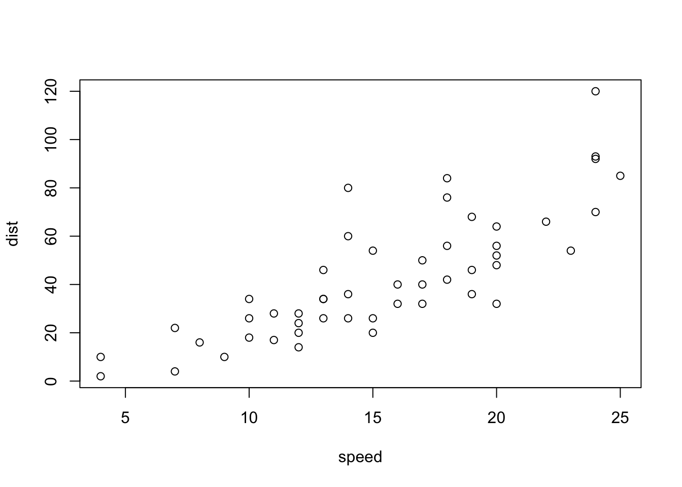

In this way you can iterate through your analytic process…switching between running code, viewing output, documenting in free text.

14.5 Workflow

Here is what I recommend for workflow:

1. Click File>New File>R Markdown to create a new file. Edit the YAML (the stuff at the top) to have the correct title, author, etc. The template that is created has some example code. Delete this generic code that is under the YAML. Save the file to your project folder.
2. Use the space under the YAML to type the objective or purpose of this analysis, and any introduction or background that is useful.
3. Carry out your analysis, inserting code chunks, running them, and documenting them with free text as you go.

• If you wish, you can see how the results look in HTML by clicking the Visual button at the top of the .

4. Sometimes we go back and re-run code in a different order, or else delete some code without re-running the entire script. This means the code is not reproducible because some objects you created no longer have code to support them. As a final check of reproducibility (the assurance that your code is self-contained and not dependent on steps you did outside the script) I recommend you always end by clicking the RUN button at the top of the panel. Specifically, choose Restart R and Run all Chunks. After it runs be sure to look at the results! This step erases all data objects in memory and starts running your script from the top. If there is an error when you do this, then something is missing in your code. Try to figure it out and make changes so that you have code in your script that does everything you expect.